
Tools for quantitative form description; an evaluation of different software packages for semi-landmark analysis
- Published
- Accepted
- Received
- Academic Editor
- Virginia Abdala
- Subject Areas
- Zoology, Anatomy and Physiology, Computational Science
- Keywords
- Geometric morphometrics, Sliding semi-landmark, Software comparison
- Copyright
- © 2015 Botton-Divet et al.
- Licence
- This is an open access article distributed under the terms of the Creative Commons Attribution License, which permits unrestricted use, distribution, reproduction and adaptation in any medium and for any purpose provided that it is properly attributed. For attribution, the original author(s), title, publication source (PeerJ) and either DOI or URL of the article must be cited.
- Cite this article
- 2015. Tools for quantitative form description; an evaluation of different software packages for semi-landmark analysis. PeerJ 3:e1417 https://doi.org/10.7717/peerj.1417
Abstract
The challenging complexity of biological structures has led to the development of several methods for quantitative analyses of form. Bones are shaped by the interaction of historical (phylogenetic), structural, and functional constrains. Consequently, bone shape has been investigated intensively in an evolutionary context. Geometric morphometric approaches allow the description of the shape of an object in all of its biological complexity. However, when biological objects present only few anatomical landmarks, sliding semi-landmarks may provide good descriptors of shape. The sliding procedure, mandatory for sliding semi-landmarks, requires several steps that may be time-consuming. We here compare the time required by two different software packages (‘Edgewarp’ and ‘Morpho’) for the same sliding task, and investigate potential differences in the results and biological interpretation. ‘Morpho’ is much faster than ‘Edgewarp,’ notably as a result of the greater computational power of the ‘Morpho’ software routines and the complexity of the ‘Edgewarp’ workflow. Morphospaces obtained using both software packages are similar and provide a consistent description of the biological variability. The principal differences between the two software packages are observed in areas characterized by abrupt changes in the bone topography. In summary, both software packages perform equally well in terms of the description of biological structures, yet differ in the simplicity of the workflow and time needed to perform the analyses.
Introduction
Because the interaction of form and function impacts performance, biological shape is under direct selection. The shape of a bone is influenced by several parameters. The evolutionary history of an organism plays an important role and often a strong phylogenetic signal is detected in bone shape (Morgan, 2009; Fabre et al., 2013a; Fabre et al., 2014a; Álvarez, Ercoli & Prevosti, 2013). Moreover, structural factors can shape bones as physical laws constrain potential shapes and their morphogenesis (e.g., Cubo, 2004; Cubo et al., 2008). For example, functional constraints imposed through differences in locomotor behavior (e.g., Fabre et al., 2013b; Álvarez, Ercoli & Prevosti, 2013) and prey capture strategy or prey size (Andersson, 2004; Meloro et al., 2008; Cornette et al., 2013) can affect bone size and shape. Additionally, mechanical loads during development (e.g., Beaupre, Orr & Carter, 1990; Bass et al., 2002) and during the lifetime of an individual (Lanyon et al., 1982; Currey, 2003) can shape bones because of bone remodeling.
Morphometric approaches have been used extensively for quantifying shape variation in biological objects including bones (Adams, Rohlf & Slice, 2004). The first paradigm, often referred to as ‘traditional morphometrics’ was based on a statistical treatment of distances or ratios (Marcus, 1990). Yet, this approach is limited as the information captured by linear measurements does not describe the whole geometry. As a consequence, the visualization of the geometry subsequent to statistical analysis is not possible and objects with different shapes can theoretically give rise to similar measurements. Additionally, many structures are difficult to measure in practice, leading to the use of measures such as maximal length which are functionally but not anatomically homologous.
These limitations have driven the development of geometric morphometrics in the 1990’s (Bookstein, 1991; Dryden & Mardia, 1993; Adams, Rohlf & Slice, 2004; Zelditch, Swiderski & Sheets, 2012). Geometric morphometrics use outline descriptors (Fourier analysis) or point coordinates (called landmarks) rather than distances to describe the geometry of biological objects. In this approach, size is explicitly defined (centroid size, sum of the squared distances of each landmark to the centroid; Bookstein, 1991) and the relative position of landmarks is conserved (Adams, Rohlf & Slice, 2004; Zelditch, Swiderski & Sheets, 2012).
Since a big part of biological variability cannot be assessed by using anatomical landmarks (biologically homologous landmarks) only, sliding semi-landmarks were developed to quantify complex shapes devoid of landmarks. Sliding semi-landmarks can be placed on curves (Bookstein, 1997; Gunz, Mitteroecker & Bookstein, 2005) and surfaces (Gunz, Mitteroecker & Bookstein, 2005). Due to the impossibility to define anatomically homologous points on curves and surfaces this approach generates landmarks that are spatially homologous after sliding (Parr et al., 2012). Sliding semi-landmarks are allowed to move on curves and surfaces in order to optimize a pre-defined criterion (Gunz & Mitteroecker, 2013). However, the choice of this criterion has been subject to debate. The most commonly used criterion is the bending energy (Skinner & Gunz, 2010; Pizzo et al., 2011; Cornette et al., 2013; Fabre et al., 2014b). The alternative involves the minimization of the Procrustes distance (Perez, Bernal & Gonzalez, 2006; Gunz & Mitteroecker, 2013). Sliding semi-landmarks are particularly well suited for the study of bones, providing descriptors of crests or outlines (curve sliding semi-landmarks; Morgan, 2009; De Groote, Lockwood & Aiello, 2010; Monteiro & Nogueira, 2010; Álvarez, Ercoli & Prevosti, 2013) and surfaces such as articular surfaces and the diaphysis of long bones (surface sliding semi-landmarks; Fabre et al., 2013a; Fabre et al., 2013b; Fabre et al., 2014b; Schlager, 2013a; Cornette et al., 2013; Morita et al., 2014; Cornette, Tresset & Herrel, 2014).
Several software packages are currently available that allow one to perform the sliding procedure in three dimensions. One of the first packages that was developed and that is still used in many studies (e.g., Kulemeyer et al., 2009; Fabre et al., 2013a; Fabre et al., 2013b; Cornette et al., 2013; Cornette, Tresset & Herrel, 2014) is ‘Edgewarp’ (Bookstein & Green, 1994). The ‘EVAN toolbox’ (http://evan-society.org) also performs sliding of semi-landmarks amongst other operations. Some authors have developed their own routines such as the Mathematica (Wolfram Inc., Modesto, California, USA) code used by Gunz & Mitteroecker (2013). Recently two R packages have been published: geomorph (Adams & Otárola-Castillo, 2013), featuring landmark placement, treatment and analysis, and ‘Morpho’ (Schlager, 2013b) featuring landmark importation from several other software packages and performing geometric morphometric treatment and analysis.
Because specimen digitization, the first step of any three dimensional surface analysis, is a time-consuming step that cannot be easily shortened, it could be of great interest to reduce the duration of the second step: the sliding procedure. The aim of the present study is to compare the workflow and the results obtained with two different software packages for the same three dimensional sliding task. We selected ‘Edgewarp’ (Bookstein & Green, 1994), an established reference for these types of analyses and ‘Morpho’ (Schlager, 2013b) a recently published set of R routines. We focused on a practical and biological test comparing a long bone in different mustelids. We followed the sliding procedure detailed in Gunz, Mitteroecker & Bookstein (2005) using both software packages. Differences between the results were examined and discussed in the light of the biological structures involved. The time required was measured for several steps and the global workflow (e.g., file handling, external software requirements) was compared.
Materials and Methods
Material
We used the humeri from 10 specimens belonging to five mustelid species (2 specimens per species; Table 1): Meles meles (Linnaeus, 1758), Mustela putorius (Linnaeus, 1758), Gulo gulo (Linnaeus, 1758), Martes martes (Linnaeus, 1758), and Enhydra lutris (Linnaeus, 1758). These species were chosen because they are widely distributed across the mustelid phylogeny and illustrate a relatively large diversity in both size, shape and ecology (Nowak, 2005; Schutz & Guralnick, 2007; Wilson et al., 2009; Hunter & Barrett, 2011). By choosing these specimens we attempted to encounter the largest number of potential pitfalls and difficulties during the sliding procedure. All specimens used are housed in the collections of ‘Mammiferes et Oiseaux’ from the Muséum National d’Histoire Naturelle in Paris, France.
| Species | Institution specimen |
|---|---|
| Martes martes | CG 1994-806 |
| CG 2005-232 | |
| Gulo gulo | CG 1983-946 |
| CG 1995-1208 | |
| Mustela putorius | CG 1991-605 |
| CG 2004-639 | |
| Meles meles | CG 2005-707 |
| CG 1987-28 | |
| Enhydra lutris | CG 1935-124 |
| A12503 |
Notes:
- CG
-
Muséum National d’Histoire Naturelle Catalogue Général, Paris, France
- A
-
Muséum National d’Histoire Naturelle Anatomie Comparée, Paris, France
3D modeling
Bones were digitized in three dimensions using a white light fringe Breuckmann 3D surface scanner (white light fringe StereoSCAN3D model with a camera resolution of five megapixels). Raw scans were treated using Geomagic (Geomagic Studio; Raindrop Geomagic, Research Triangle Park, North Carolina, USA) to fill-in remaining holes and to remove highly creased edges and spikes. Next, models were decimated to contain 100,000 triangles resulting in homogeneous 3D surface models. The number of triangles was arbitrarily fixed to generate models that are not too cumbersome, but without altering the geometry of the object. The models were converted to ‘.sur’ using the ‘obj2sur’ tool provided at ‘ ftp://brainmap.stat.washington.edu/edgewarp/utils/’ in order to import them into ‘Edgewarp.’
3D anatomical landmark and curve digitization
Landmarks and curves were digitized on the surfaces of the scans using the Landmark software package (Wiley et al., 2005). Twenty-seven 3D homologous anatomical landmarks were chosen and are visible on all specimens (Fig. 1 and Table 2). Eighteen 3D curves were defined at the margins of articular surfaces and along crests. All curves are bordered by anatomical landmarks as recommended by Gunz, Mitteroecker & Bookstein (2005). The curves were digitized with a high density of points (40–160 points per curve depending on the curve length) and then sub-sampled to the number listed in Table 3. This dataset was then used to perform an identical sliding procedure using both ‘Edgewarp’ and ‘Morpho.’

Figure 1: 3D view of a Martes martes MNHN 2005-232 humerus showing the location of the 27 anatomical landmarks and 18 curves used to quantify the humeral shape.
(A) caudal; (B) cranial; (C) lateral views. Red: anatomical landmarks. Blue: curve sliding semi-landmarks. Yellow: surface sliding semi-landmarks. See Table 2 for landmark definitions.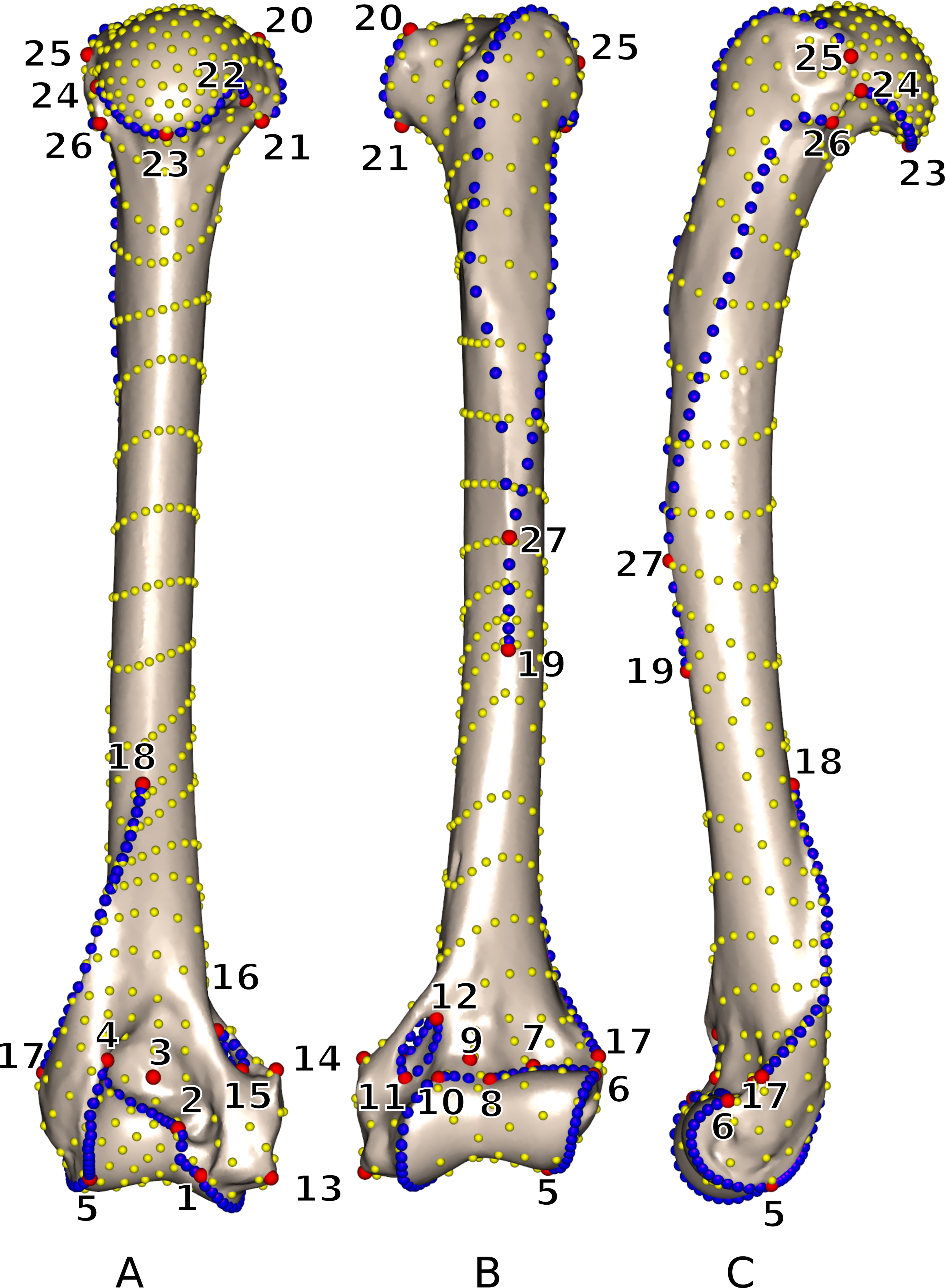
| LM | Definition |
|---|---|
| 1 | Most disto-medial point of the trochlea |
| 2 | Most medio-proximal point of the caudal side of the trochlea |
| 3 | Point of maximum of curvature of the olecranon fossa |
| 4 | Most latero-proximal point of the caudal side of the trochlea |
| 5 | Most distal point of contact between the trochlea and the capitulum |
| 6 | Most latero-proximal point of the cranial side of the capitulum |
| 7 | Point of maximum of curvature of the radial fossa |
| 8 | Maximum concavity of the cranial margin of the trochlea |
| 9 | Point of maximum of curvature of the coronoid fossa |
| 10 | Most medio-proximal point of the cranial side of the trochlea |
| 11 | Most distal point of the cranial side of the supracondylar foramen |
| 12 | Most proximal side of the cranial side of the supracondylar foramen |
| 13 | Most distal tip of the medial epicondyle |
| 14 | Most proximal tip of the medial epicondyle |
| 15 | Most distal point of the caudal side of the supracondylar foramen |
| 16 | Most proximal point of the caudal side of the supracondylar foramen |
| 17 | Most disto-cranial point of the lateral epicondylar crest |
| 18 | Most proximal point of the lateral epicondylar crest |
| 19 | Most distal point of the deltopectoral crest |
| 20 | Upper tip of the lesser tuberosity |
| 21 | Most disto-medial point of the lesser tuberosity |
| 22 | Most medio-caudal point of contact between the lesser tuberosity and humeral head |
| 23 | Disto-caudal tip of the humeral head |
| 24 | Latero-caudal point of contact between the greater tuberosity and the humeral head |
| 25 | Most antero-proximal point of the greater tuberosity crest |
| 26 | Tip of the tuberosita teres minor |
| 27 | Contact point between tricipital line and greater trochanter crest |
Notes:
- LM
-
landmark index
A semi-automatic point placement was used to place surface semi-landmarks on the scans. A template was modeled using the Blender software (Blender Online Community, 2014) following the procedure described in Souter et al. (2010). We created a mesh of 598 points representing a simplified form of the humerus. Landmarks and curves were digitized on the template surface as it was done on the actual scans of the specimens. Then in both ‘Edgewarp’ and ‘Morpho,’ landmarks and curves were used to compute a thin plate spline (TPS) deformation of the template. Next, surface sliding landmarks were projected from the deformed template onto the bone surface (Gunz & Mitteroecker, 2013). In summary, the template used in this study contains a total of 817 points including 27 3D homologous anatomical landmarks, 192 sliding semi-landmarks on curves and 598 sliding semi-landmarks on surfaces.
The sliding procedure was performed following the algorithm detailed in Gunz, Mitteroecker & Bookstein (2005). Four TPS relaxations were performed, the first TPS relaxation was performed against the template, the three others against Procrustes consensus calculated using the data from the previous iteration.
Time estimation
The time for surface pre-processing and initial projection was measured by the value displayed in ‘Edgewarp’ log. The time required by ‘Edgewarp’ for the three iterations of sliding against Procrustes consensus was measured using a timer. The time required to run the ‘Morpho’ package in R was assessed by running the timestamp R function at the beginning and end of tasks and calculating the difference. These durations do not include time required for writing the script (scripts for data formatting for ‘Edgewarp’, and R scripting for ‘Morpho’). All analyses were run on a laptop computer (Asus k55vj) with a Intel® i7-3630QM CPU, 4 Gb of memory, running on Linux Ubuntu V14.04.
Geometric morphometrics and visualization
Data analysis and visualization were performed using the R software (R Core Team, 2014). In order to superimpose geometries and isolate size and shape, a generalized Procrustes analysis (GPA) was performed (Gower, 1975; Rohlf & Slice, 1990; Dryden & Mardia, 1998) for the ‘Edgewarp’ and the ‘Morpho’ dataset separately using the ‘Rmorph’ package (Baylac, 2013). We reduced dimensionality of the datasets by keeping the nine first non-null axes of a Principal Component Analysis (PCA) performed on the coordinates in the tangent space. In order to asses differences between the dataset produced by each software, a PROTEST analysis was performed using the ‘vegan’ package (Oksanen et al., 2015) run with 100,000 iterations (Peres-Neto & Jackson, 2001). The ‘vegan’ package was then used to draw the Procrustean superimposition plot. The three dimensional visualization of bone surfaces, landmarks, and vectors between homologous points were performed using the ‘rgl’ (Adler & Murdoch, 2012) and ‘Morpho’ (Schlager, 2013b) packages in R.
Results
Global shape variability
The PROTEST analysis highly supports the congruence of the two datasets (m12 = 0.00325; P < 10−5). The Procrustean superimposition plot (Fig. 2) shows the differences between the two datasets. It becomes immediately clear that the between-methods variability is smaller than the inter-specimens variability, even within species. The Procrustes residuals of specimens analyzed with both methods vary from one specimen to the other (Table 4). The specimens showing the maximal Procrustes residuals are Gulo gulo 1983-946, Mustela putorius 1991-605, and Enhydra lutris 1935-124 (respectively c, e, and i; Fig. 2). The first axis separates Enhydra lutris (i and j; Fig. 2) and Martes martes (a and b; Fig. 2). On the two first axes Mustela putorius and Gulo gulo show intra-specific distances greater than the inter-specific ones with Mustela putorius 2004-639 (f; Fig. 2) being closer to Gulo gulo 1995-1208 (d; Fig. 2) than to Mustela putorius 1991-605 (e; Fig. 2) and Gulo gulo 1983-946 (c; Fig. 2) being closer to Mustela putorius 1991-605 (e; Fig. 2) than to Gulo gulo 1995-1208 (d; Fig. 2).
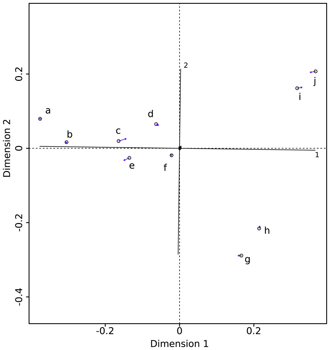
Figure 2: Procrustes superimposition of the Morpho (circles) and Edgewarp (arrow heads) results. Arrows present Procrustes residuals.
(a) Martes martes 2005-232; (b) Martes martes 1994-806; (c) Gulo gulo 1983-946; (d) Gulo gulo 1995-1208; (e) Mustela putorius 1991-605; (f) Mustela putorius 2004-639; (g) Meles meles 2005-707; (h) Meles meles 1987-28; (i) Enhydra lutris 1935-124; (j) Enhydra lutris A12503.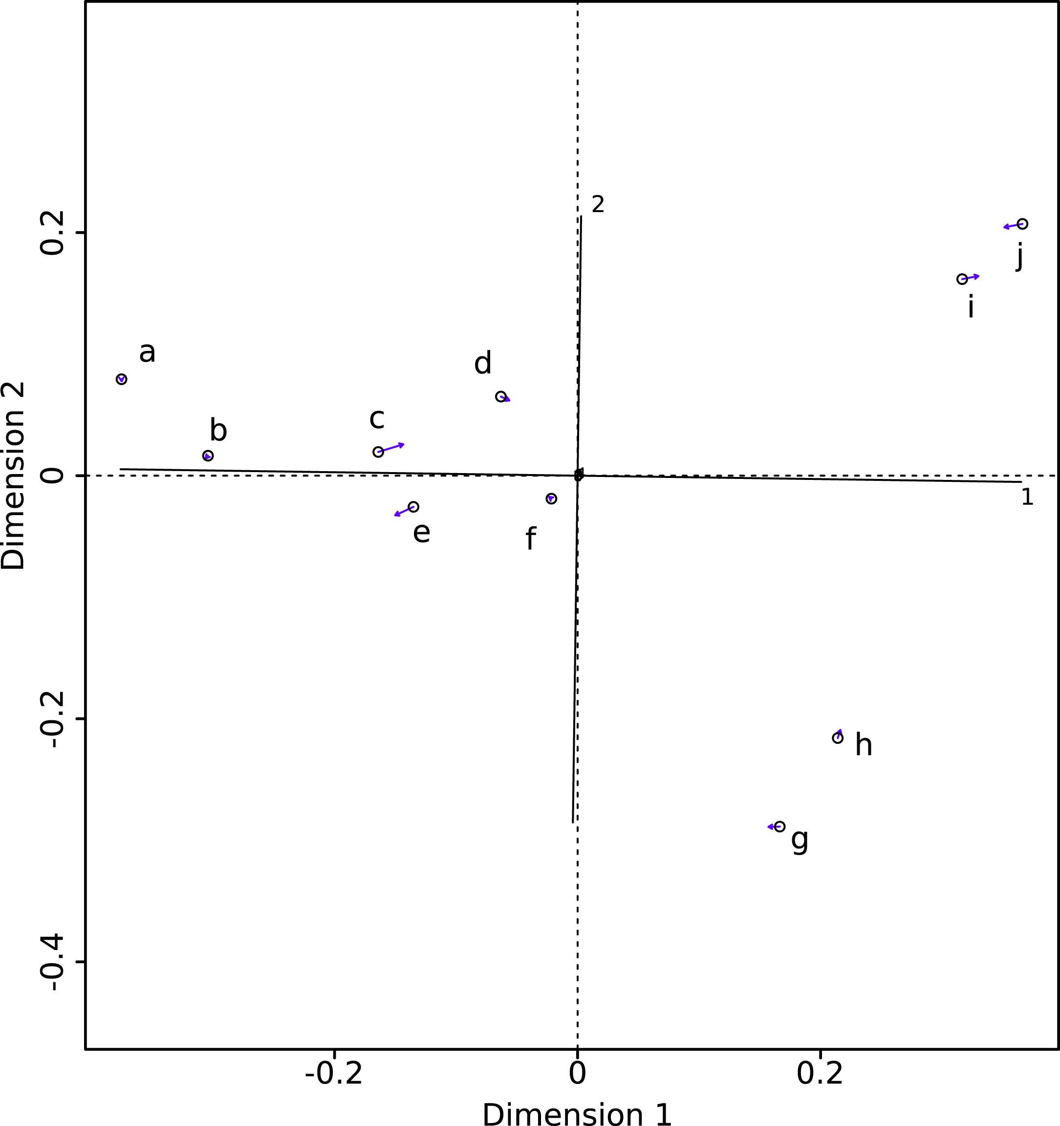
| Init LM | Term LM | NbSl |
|---|---|---|
| 1 | 2 | 5 |
| 2 | 4 | 10 |
| 4 | 5 | 15 |
| 5 | 6 | 15 |
| 6 | 8 | 10 |
| 8 | 10 | 3 |
| 10 | 1 | 15 |
| 11 | 12 | 5 |
| 12 | 11 | 5 |
| 15 | 16 | 5 |
| 16 | 15 | 5 |
| 17 | 18 | 23 |
| 20 | 21 | 5 |
| 22 | 23 | 10 |
| 23 | 24 | 9 |
| 25 | 27 | 26 |
| 26 | 27 | 21 |
| 27 | 19 | 5 |
Notes:
- init LM
-
initial anatomical landmark index
- term LM
-
terminal anatomical landmark index
- NbSl
-
number of curve sliding semi-landmarks
| Specimen | Procrustes residuals |
|---|---|
| Enhydra lutris 1935-124 | 0.020489693 |
| Enhydra lutris A12503 | 0.017785627 |
| Gulo gulo 1983-946 | 0.037204213 |
| Gulo gulo 1995-1208 | 0.010347460 |
| Martes martes 1994-806 | 0.009211963 |
| Martes martes 2005-232 | 0.015334387 |
| Meles meles 1987-28 | 0.008102059 |
| Meles meles 2005-707 | 0.011307574 |
| Mustela putorius 1991-605 | 0.021816036 |
| Mustela putorius 2004-639 | 0.005777793 |
Differences between mean shapes
The middle part of the greater trochanteric crest (2 in Fig. 3) presents the strongest differences. The neighboring points on the surface of the greater trochanteric crest are also affected. The second most variable area is the curve sliding around the cranial side of the medial supracondylar foramen (1 in Fig. 3) at the latero-distal part. Additionally, a point on the diaphysis located on the disto-medial side of the greater trochanter crest varies considerably.
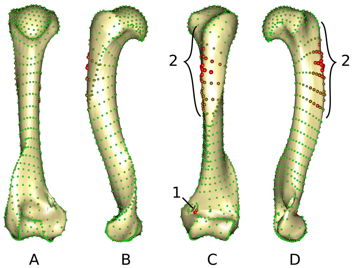
Figure 3: Warped mesh calculated on the Procrustes mean shape showing the most varying areas.
(A) caudal; (B) lateral; (C) cranial; (D) medial views. Sphere colors (from green to red) and size are proportional to the Euclidean distance between points in the Procrustes mean shape for each software output after sliding. Points showing the maximal distance between the results obtained by the two software packages are large red points (as opposed to minimal distances being represented by small green points). 1: cranial side of the medial supracondylar foramen; 2: greater trochanteric crest.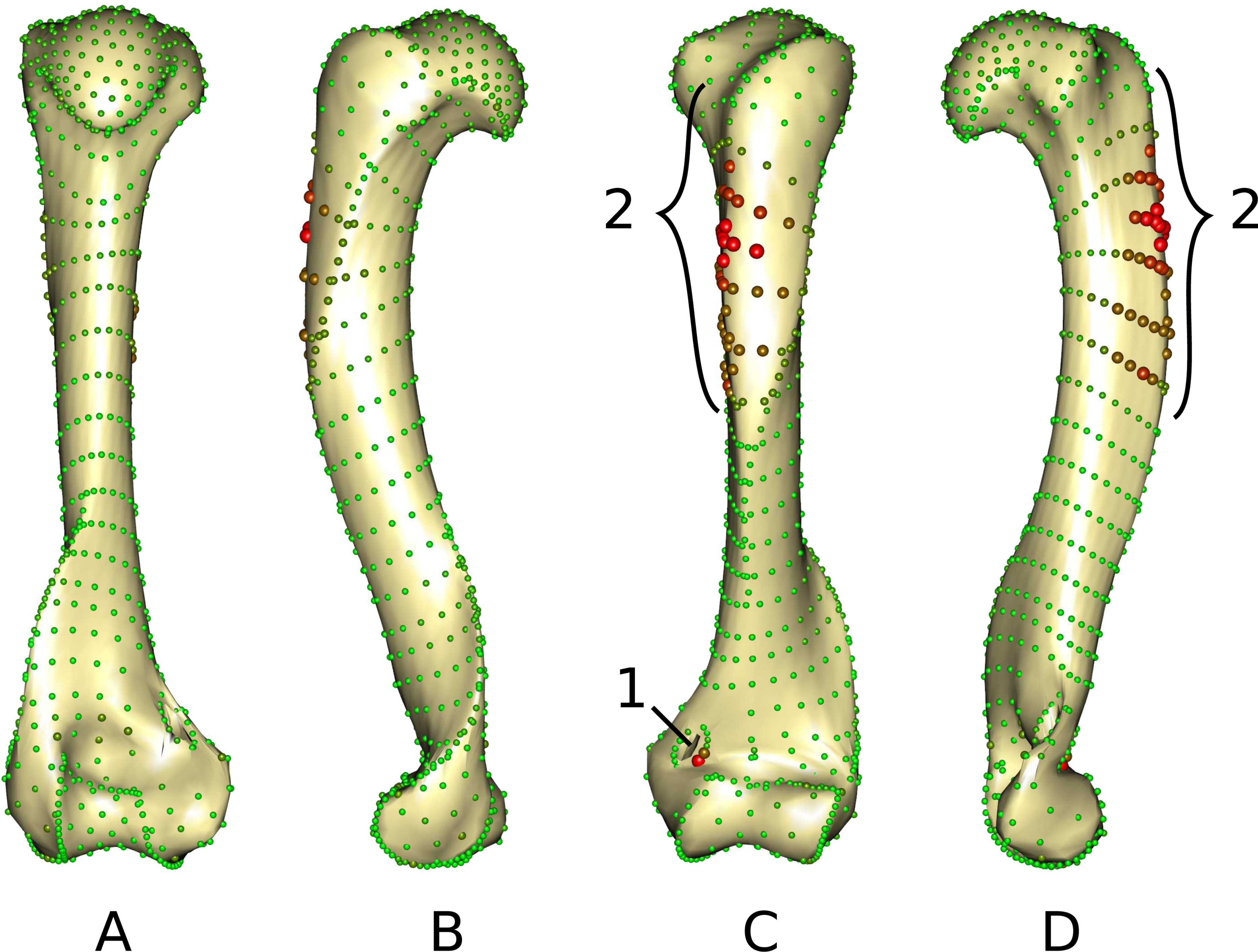
The most variable specimens
As highlighted in Fig. 2 and Table 4, differences linked to the software are more important in some specimens than in others. Gulo gulo 1983-946, Mustela putorius 1991-605, and Enhydra lutris 1935-124 display the largest differences between methods (Table 4). Beyond the differences noted in the mean shapes, we investigated the ones specific to each of these specimens. Gulo gulo 1983-946 (Figs. 4A) presents a displacement of points located on the deltoid crest, more specifically around the insertion of an ossified tendon (teres major/latissimus dorsi). The most variable point switches from one side of this structure to the other depending on the software used, suggesting that one of the methods did not succeed in sliding the point across this structure. Mustela putorius 1991-605 (Fig. 4B) presents a point shifting from one side to the other side of the crest on the diaphysis distal to the lesser trochanter. The ‘Edgewarp’ points (yellow) are located on the caudal side of the crest whereas the ‘Morpho’ points (blue) are located on the cranial side. Enhydra lutris 1935-124 (Fig. 4C) presents a variation associated with a small depression located medially to the deltoid crest. ‘Edgewarp’ points (yellow) slide on the distal margin of the foramen whereas the ‘Morpho’ points (blue) are close to the cranial margin of the depression. Surrounding points are also affected. The most variable points around the supracondylar foramen, at the latero-distal part of its cranial side are driven by the Meles meles 1987-28. For this specimen ‘Edgewarp’ points are concentrated on the most proximal part of this curve whereas ‘Morpho’ points are located more distally.
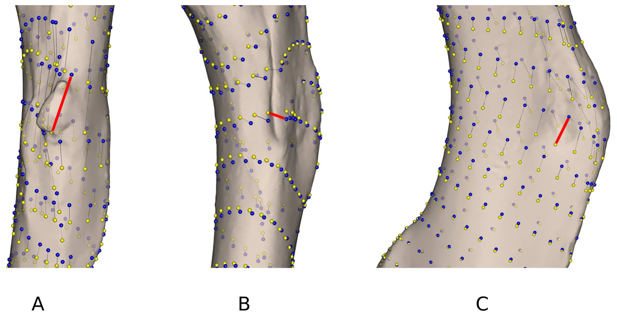
Figure 4: Close up view of the most variable areas of some specimens after sliding.
Yellow: ‘Edgewarp’; blue: ‘Morpho’; black vectors link the homologous points in the output of each software package; the red vectors highlight the most variable points. (A) Gulo gulo 1983-946 medio-cranial view of the greater trochanteric crest; (B) Mustela putorius 1991-605 medio-caudal view of the lesser trochanter (distal) crest along the diaphysis. (C) Enhydra lutris 1935-124 medial view of the distal part of the greater trochanteric crest.
Time
The times measured for surface pre-processing, the initial point projection, and the relaxations against the Procrustes mean shape, iterated three times, are given in Table 5. ‘Morpho’ requires a much shorter time compared to ‘Edgewarp’. The time required for the sliding against Procrustes mean shape by ‘Edgewarp’ is moreover an active time, meaning that the user needs to run each step of the iterations manually. This part also requires the computation of the GPA which is not implemented internally in ‘Edgewarp’. Based on the results of the GPA, new input files must be generated prior to performing the next iteration.
| Edgewarp | Morpho | % | |
|---|---|---|---|
| Surface pre-processing (s) | 1,320 | 4 | 0.3 |
| Initial point projection (s) | 600 | 20 | 3.3 |
| Sliding against mean shape 3 iterations (min) | 105 | 2 | 1.9 |
Notes:
%, percentage of time required by ‘Morpho’ compared to ‘Edgewarp.’
Discussion
General variability
The distribution of specimens in morphological space is similar, irrespective of the software used. The biological information is similarly described with both packages and thus both can be used to describe complex biological shapes without an inherent bias. Nevertheless, as some local divergence between methods can be observed, results could differ for intra-specific studies often describing more subtle shape variations. The morphospace obtained after sliding is structured by the most extreme ecological niches in our sample suggesting that functional constraints drive much of the shape variability. The first dimension of the Procrustean superimposition plot separates Enhydra lutris and Meles meles (respectively i, j and g, h Fig. 2) from the other species. The maximal distance on this axis is obtained between Enhydra lutris (i and j, Fig. 2) which is the most aquatic of the Mustelidae sampled here (Estes, 1980; Bodkin, 2001) and Martes martes (a and b, Fig. 2) which is the most arboreal (Nowak, 2005) species in our sample. The second dimension of the Procrustean superimposition plot separates Meles meles (g and h, Fig. 2), the only semi-fossorial species in our sample (Nowak, 2005) from Enhydra lutris (i and j). Phylogeny, size and/or body mass (allometry) have been shown to be important factors shaping the humerus in Carnivora (Heinrich & Biknevicius, 1998; Fabre et al., 2013a; Martín-Serra, Figueirido & Palmqvist, 2014). Our data suggest that life-style is indeed an important driver of forelimb shape in mustelids. Nevertheless, this is a small sample only and these results should be interpreted with caution.
Differences
As they are computed from the same dataset, morphospaces obtained by the two software where expected to be the same. The two morphospaces (relative distances between specimens) are indeed generally similar, which is validated by the significant PROTEST. Nevertheless some specimens show slightly different positions in the morphospace depending on the software (Gulo gulo 1983-946, Mustela putorius 1991-605, and Enhydra lutris 1935-124, respectively c, e, and i; Fig. 2). Specimens showing the greatest variation in their relative position between the two software are bones with areas where a structure interrupts the main curvature of the surface resulting in strong local deformations (Fig. 4). The fact that these local deformations are of a size similar to the distance between surface sliding landmarks appears to play a role. Indeed, highly curved structures can “puncture” the meshing constituted by the surface sliding semi-landmarks. Even if concerning only few points, these structures can lead to displacement of the specimen into the morphospace and could consequently have an impact in the biological interpretation of the morphospace (i.e., modifying phenetic affinities; Fig. 2). A greater number of surface sliding semi-landmarks in these specific areas could allow points to slide at the surface of a structure. Additionally, if the aforementioned structures present no biological meaning for the study, an a priori elimination could avoid giving too much weight to these structures in the analysis. Small foramina and ossified tendon insertions could be removed prior to the sliding procedure using dedicated tools in meshing software.
The differences observed between the two datasets thus likely result from differences during the sliding process at particular points of some specimens rather than reflect a global difference between methods. Such differences could be a consequence of differences between the two software packages in the computation of the relaxation as well as in the computation of the projection of the points on the surface of the specimen. Consequently mixing in a single analysis results obtained by the two software should be avoided.
Time
‘Edgewarp’ appears more time-consuming than ‘Morpho’ for the same sliding task. ‘Edgewarp’ requires 30–300 times the time required by ‘Morpho’ for the same tasks. Two reasons can be put forward to explain these differences: computational efficiency and workflow complexity. ‘Edgewarp’ is a non-parallelized software whereas many ‘Morpho’ functions can be run on several cores, thus improving processing time. The effect of computation power remains low on a small dataset like the one presented here, but can lead to a considerable time difference in the case of the analysis of larger datasets. In addition to the number of steps constituting the workflow, the number of actions performed by the user should also be taken into consideration. The use of ‘Edgewarp’ requires one to open each surface, curve, and landmark file manually. The subsequent iterative relaxation requires several manual operations per iteration as does the data saving after sliding. The use of a programming language such as python (Van Rossum & De Boer, 1991), bash (Free Software Foundation, 2013), or even R (R Core Team, 2014) is useful to automate some parts of the workflow such as the ‘.sav’ generation. Once written, scripts can be run several times or adapted, reducing the time required to perform these repetitive tasks. Furthermore ‘Edgewarp’ does not perform the Procrustes superimposition needed for the computation of the mean shape, entailing the use of another software package (here R with the ‘Rmorph’ library). Therefore the time needed cannot be spent doing other things. Conversely using ‘Morpho,’ the principal active component is the writing of the script. Computation can then be run as a background task or on a remote computer. This is an advantage as much for an initial analysis of the data as for modifications (for example adding specimens or correcting a landmark placement).
Problems encountered
Deviations from the initial curves were observed in ‘Morpho.’ This deviation from the initial curve is a logical consequence of the relaxation procedure along tangents. Surface sliding semi-landmarks tend to move inside or outside the volume of the specimen depending on the local curvature as they are sliding on the tangent (Gunz, Mitteroecker & Bookstein, 2005). Curve sliding landmarks move outside of the curve on the opposite side of the center of curvature. This is why points are projected back onto the surface after relaxation. But in some cases such as for the greater trochanteric crest (2 in Fig. 3) of Gulo gulo and Martes martes this leads to deviations of the curve from its initial position. This effect is counter balanced in ‘Edgewarp’ by re-projecting points onto the ‘rail.’ This ‘rail’ (named ‘.cur’ in ‘Edgewarp’) is constituted of a collection of points digitized on the bone surface, linked by segments. Consequently the definition of the ‘rail’ needs a large number of points to achieve a good description. However, when two curves are close, points can ‘jump’ from one curve to the other if the relaxed position is close to the second curve. Two strategies can counterbalance this effect in ‘Morpho’; first using a higher density of curve sliding landmarks (Gunz, Mitteroecker & Bookstein, 2005) and second, by reducing the relaxation step size. This last solution presents the advantage of being applicable on the initial dataset and does not require new data collection.
We also noticed points being projected on the wrong side of the supracondylar lateral crest and points projecting through bone from the olecranon fossa to the coronoid fossa while using ‘Edgewarp.’ The projection of surface sliding semi-landmarks from the template to the specimen surface is a crucial step preceding the actual sliding process. The main principle used in both software packages is a TPS deformation of the template constrained by anatomical and curve sliding landmarks followed by a projection onto the specimen surface. For some areas such as the lateral supracondylar crest, surface points can be projected onto the wrong side of the crest, if projected to the closest surface after TPS deformation. The ‘Morpho’ function ‘placePatch’ implements additional steps to avoid such effects. Inflation/deflation along the normals (vector giving the orientation of the mesh vertex) is performed; then the normals of projected points are compared to those of the template to avoid inside-out effects. In ‘Edgewarp,’ the graphical interface allows users to manually displace and correct wrongly projected points. The ‘Morpho’ strategy presents the advantage to be automated and integrated as a part of the ‘placePatch’ function. In contrast, ‘Edgewarp’ requires the manual displacement of the points, implying the correct identification of wrongly projected points prior to moving them to the correct side. This requires the investigation of all points on every specimen which is time consuming. The use of surface sliding semi-landmarks at the very vicinity of the curves appears to be a factor leading to projection on the wrong side of crests. Therefore, this problem could be circumvented by taking this fact into account during the design of the template.
Aside of the own properties of these software, the help file determines a part of the global ergonomy of any software package. Edgewarp’s user manual (User’s manual, EWSH3.19; available at ftp://brainmap.stat.washington.edu/edgewarp/) was last updated on March 2002. Additionally, it remains apparently unfinished as indicated by the author’s comments appearing along the text. On the other hand, Morpho’s help file is frequently updated and examples are provided for each function.
Conclusions
This study shows that the results obtained by two software packages for 3D shape quantification, ‘Edgewarp’ (Bookstein & Green, 1994) and ‘Morpho’ (Schlager, 2013b), are similar and that biological variability is similarly described by both software packages. We highlight the fact that small structures jutting out of the surface as well as depressions may have an impact on the results and underline the importance of identifying these structures prior to the sliding operation. An increase in the density of the surface sliding landmarks in these areas or the removal of structures that do not contain biologically relevant information for the study are possible solutions for avoiding strong impact of these structures on the morphospace. The present study focuses on a small number of species, showing a large range of size and shape variation. This experimental design highlights the kind of structures that drive divergence between the two software packages. However, this design does not allow us to anticipate possible biases for different datasets such as those used in intra-specific studies where the variability between specimens is often quite subtle. Beyond the similarity in results, ‘Morpho’ is faster than ‘Edgewarp’ for the same sliding task, notably as a result of the computational power of ‘Morpho’ and the complexity of the workflow in ‘Edgewarp.’ ‘Edgewarp,’ on the other hand provides a visual approach to the sliding procedure. Thanks to the exploitation of modern computational power, ‘Morpho’ library, provides a powerful tool for the treatment of larger datasets.