Generating Faces with Torch
In this blog post we’ll implement a generative image model that converts random noise into images of faces! Code available on Github.
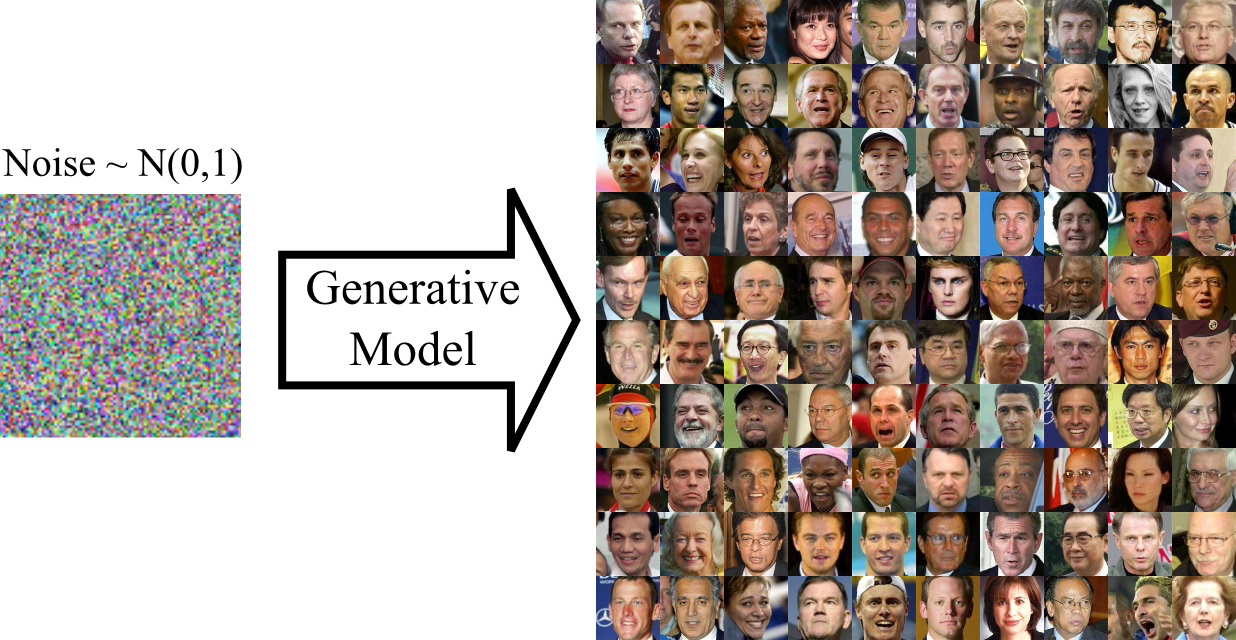
For this task, we employ a Generative Adversarial Network (GAN) [1]. A GAN consists of two components; a generator which converts random noise into images and a discriminator which tries to distinguish between generated and real images. Here, ‘real’ means that the image came from our training set of images in contrast to the generated fakes.
To train the model we let the discriminator and generator play a game against each other. We first show the discriminator a mixed batch of real images from our training set and of fake images generated by the generator. We then simultaneously optimize the discriminator to answer NO to fake images and YES to real images and optimize the generator to fool the discriminator into believing that the fake images were real. This corresponds to minimizing the classification error wrt. the discriminator and maximizing it wrt. the generator. With careful optimization both generator and discriminator will improve and the generator will eventually start generating convincing images.
Implementing a GAN
We implement the generator and discriminator as convnets and train them with stochastic gradient descent.
The discriminator is a standard convnet with consecutive blocks of convolution, ReLU activation, max-pooling and dropout.
model_D = nn.Sequential()
model_D:add(cudnn.SpatialConvolution(3, 32, 5, 5, 1, 1, 2, 2))
model_D:add(cudnn.SpatialMaxPooling(2,2))
model_D:add(cudnn.ReLU(true))
model_D:add(nn.SpatialDropout(0.2))
model_D:add(cudnn.SpatialConvolution(32, 64, 5, 5, 1, 1, 2, 2))
model_D:add(cudnn.SpatialMaxPooling(2,2))
model_D:add(cudnn.ReLU(true))
model_D:add(nn.SpatialDropout(0.2))
model_D:add(cudnn.SpatialConvolution(64, 96, 5, 5, 1, 1, 2, 2))
model_D:add(cudnn.ReLU(true))
model_D:add(cudnn.SpatialMaxPooling(2,2))
model_D:add(nn.SpatialDropout(0.2))
model_D:add(nn.Reshape(8*8*96))
model_D:add(nn.Linear(8*8*96, 1024))
model_D:add(cudnn.ReLU(true))
model_D:add(nn.Dropout())
model_D:add(nn.Linear(1024,1))
model_D:add(nn.Sigmoid())
This is a pretty standard architecture. The discriminator takes a 64x64 RGB image as input and predicts YES or NO with a single sigmoid output.
The generator goes in the opposite direction. We start with a small image which is upsampled and convolved repeatedly:
x_input = nn.Identity()()
lg = nn.Linear(opt.noiseDim, 128*8*8)(x_input)
lg = nn.Reshape(128, 8, 8)(lg)
lg = cudnn.ReLU(true)(lg)
lg = nn.SpatialUpSamplingNearest(2)(lg)
lg = cudnn.SpatialConvolution(128, 256, 5, 5, 1, 1, 2, 2)(lg)
lg = nn.SpatialBatchNormalization(256)(lg)
lg = cudnn.ReLU(true)(lg)
lg = nn.SpatialUpSamplingNearest(2)(lg)
lg = cudnn.SpatialConvolution(256, 256, 5, 5, 1, 1, 2, 2)(lg)
lg = nn.SpatialBatchNormalization(256)(lg)
lg = cudnn.ReLU(true)(lg)
lg = nn.SpatialUpSamplingNearest(2)(lg)
lg = cudnn.SpatialConvolution(256, 128, 5, 5, 1, 1, 2, 2)(lg)
lg = nn.SpatialBatchNormalization(128)(lg)
lg = cudnn.ReLU(true)(lg)
lg = cudnn.SpatialConvolution(128, 3, 3, 3, 1, 1, 1, 1)(lg)
model_G = nn.gModule({x_input}, {lg})
To generate an image we feed the generator with noise distributed N(0,1). After successful training, the output should be meaningful images!
local noise_inputs = torch.Tensor(N, opt.noiseDim)
noise_inputs:normal(0, 1)
local samples = model_G:forward(noise_inputs)
Balancing the GAN game
In principle, the GAN optimization game is simple. We use binary cross entropy to optimize the parameters in the discriminator. Afterwards we use binary cross entropy to optimize the generator to fool the discriminator. That said, you often find yourself left with not very convincing outputs from generator:
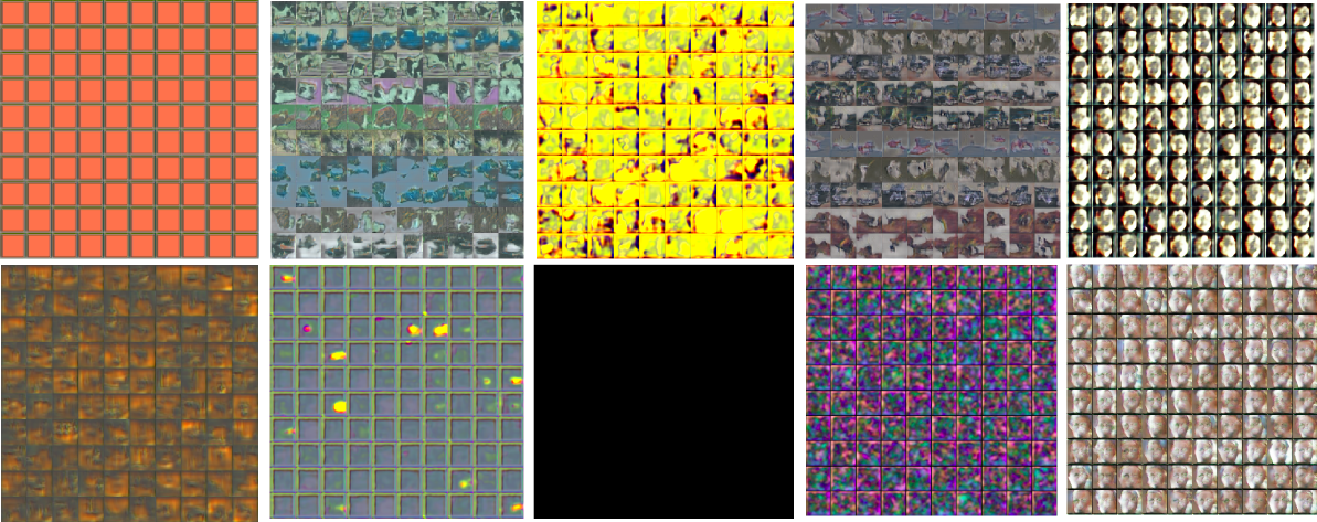
This gibberish is typical for a generator trained without proper care!
A couple of tricks are necessary for to facilitate training: First off, we need to make sure that that neither the generator nor the discriminator becomes too strong compared to the other. If the discriminator ‘wins’ and classifies all images correctly, the error signal will be poor and the generator will not be able to learn from it. Conversely, if we allow the generator to win, it is usually exploiting a non-meaningful weakness in the discriminator (e.g. by coloring the entire image blue) which is not desirable.
We monitor the training by plotting three quantities:
- How good the generator is at at fooling the discriminator (gen)
- How good the discriminator is at classifying fakes as fakes (fake)
- How good the discriminator is at classifying real images as real (real)
Below we plot these quantities during trained for three separate networks. In panel A) we have made the discriminator too powerful by adding batch normalization layers. The training never converges because the sigmoid saturates resulting in a poor error signal for backpropagation.
To alleviate the problem, we monitor how good the discriminator is at classifying real and fake images and how good the generator is at fooling the discriminator. If one of the networks is too good, we skip updating its parameters according to the following rules. The convergence is shown in panel B). We also removed batch normalization from the discriminator.
local margin = 0.3
     sgdState_D.optimize = true
     sgdState_G.optimize = true
if err_F < margin or err_R < margin then
     sgdState_D.optimize = false
end
if err_F > (1.0-margin) or err_R > (1.0-margin) then
     sgdState_G.optimize = false
end
if sgdState_G.optimize == false and sgdState_D.optimize == false then
     sgdState_G.optimize = true
     sgdState_D.optimize = true
end
It seems a bit wasteful to not update the parameters in every batch. We therefore try another heuristic based on regularization of the discriminator if the generator is performing poorly. We increment the discriminators L2 penalty if the generator is not within a target range. If the generator fools the discriminator in 50% of the cases the error would be ~log(0.5) ~=0.69. We set the target range to be 0.9-1.2 i.e the discriminator should be better than the generator but not too much. The training is shown in panel C) (Keep in mind that the x-axis is different)
if f > 1.3 then  -- f is generator error
sgdState_D.coefL2 = sgdState_D.coefL2 + 0.00001
end

if f < 0.9 then
sgdState_D.coefL2 = sgdState_D.coefL2 - 0.00001
end

if sgdState_D.coefL2 < 0 then
sgdState_D.coefL2 = 0
end
<img src="https://raw.githubusercontent.com/torch/torch.github.io/master/blog/_posts/images/monitor.png", width="90%">
These simple heuristics seem to work, but there is definitely room for improvement. Most importantly, they allows us to crank up the learning rate and use RMSProp.
A few other tricks are necessary for successful GAN training:
-
Batch normalization speeds up training a lot when used in the generator. Using batch normalization in the discriminator is dangerous as the discriminator becomes too powerful.
-
Plenty of dropout is needed in the discriminator to avoid oscillating behavior caused by the generator exploiting a weakness of the discriminator. Dropout can also be used in the generator.
-
It may be beneficial to limit the capacity of the discriminator. This is done by decreasing its number of features such that the generator contains more parameters.
We have created a video that that shows what the model generates during the first three epochs of training. In our experience you should not be too worried if the model initially generate very colorful non-sense but the model is probably wrong if all generated images are equal or nearly equal.
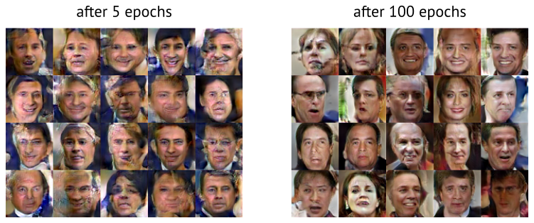
Generating faces
We train our GAN using aligned and cropped images from the Labeled faces in the wild dataset. After at around 5 epochs (around 30 minutes on a GPU) you should start to see some spooky faces (left). And after 100 epochs will look more pleasant (right).
After a day of training, we get decent looking walks around in the latent space of the GAN (full movie on YouTube):
Going Further
While it is good fun to generate images from noise, GANs gives us no control over the latent space.
A related generative model is the Variational autoencoder (VAE) [3] in which the decoder maps samples from a prior distribution to dataset samples - very similar to the GAN generator.
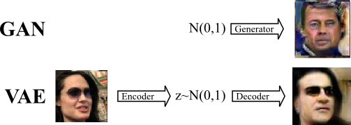
The VAE decoder is trained differently as we seek to minimize the pixelwise reconstruction error of the decoded image compared to the encoded image. This error term is problematic for images since translation is punished disproportionately to the small error perceived by human vision. In practice, this means that VAEs are biased towards generating smooth images with a correct global subject whereas GAN generated images have more correct local style with less emphasis on the global structure.
Here is an example of VAE images generated from random samples z ~ N(0,1):
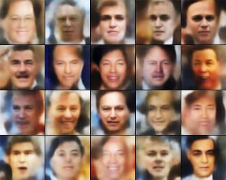
Though the images clearly contain faces, they are somewhat boring because of their smoothness. To improve this, we try to combine VAE and GAN in one model:

We let the GAN and the VAE share latent space z ~ N(0,1) as well as the decoder/generator network. We combine the error terms when training the model:
Error = [VAE prior] + [VAE reconstruction error] + [GAN error]
To optimize the parameters of the combined model, we minimize the VAE terms while balancing the GAN term as already described. The gradients to the decoder/generator parameters are weighted to ensure a sensible contribution from both models.
Below we show images generated by the VAE/GAN model.
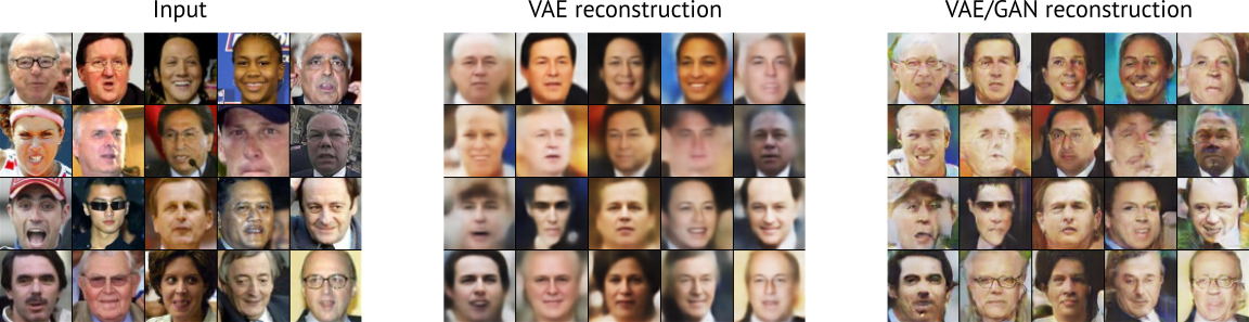
Compared to the plain VAE, the VAE/GAN images are more interesting as they contain more details. Most notably, VAE/GAN has learned to reconstruct a pair of glasses.
Conclusion
Getting a GAN to train successfully can be extremely hard. In this blog we have shared a few do and don’t’s when training the GAN. Finally we have shown that GAN and VAE’s can be combined into an interesting model. Future work will show if this combination can improve e.g. semi-supervised learning.
Acknowledgements
Eyescream authors [2] for making their code public. Our code is heavily based on the CIFAR code released for the LAPGAN paper[2].
Torch VAE from Y0st: https://github.com/y0ast/VAE-Torch
References
[1] Goodfellow, Ian, et al. “Generative adversarial nets.” Advances in Neural Information Processing Systems. 2014.
[2] Denton, Emily, et al. “Deep Generative Image Models using a Laplacian Pyramid of Adversarial Networks.” arXiv preprint arXiv:1506.05751 (2015).
[3] Kingma, Diederik P., and Max Welling. “Auto-encoding variational bayes.” arXiv preprint arXiv:1312.6114 (2013).
comments powered by Disqus